Up: Logistic Growth Model
One-Dimensional Dynamical Systems
Part 2: Logistic Growth Model
Visualizing an orbit
Let us consider the evolution for p0 = 12, under
the assumption that the university campus provides essential needs for
maximally E = 200 squirrels. We set
 = 2, which
corresponds to a growth rate of 1 baby per squirrel each year. What do
you expect to happen as the years go by? We can visualize the orbit of
p0 = 12 by plotting the iterates
pn against the years n. In the
following picture the evolution is shown over 100 years.
= 2, which
corresponds to a growth rate of 1 baby per squirrel each year. What do
you expect to happen as the years go by? We can visualize the orbit of
p0 = 12 by plotting the iterates
pn against the years n. In the
following picture the evolution is shown over 100 years.
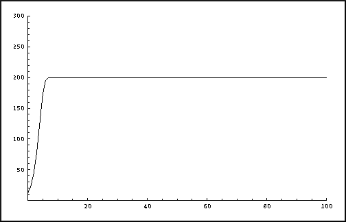
Logistic growth with growth factor
= 2.
The picture shows a monotonic increase towards the saturation value
E. It is suprising to see what happens if we vary
, but still use
E = 200 and p0 = 12. The following two
pictures show the results over 100 years for
= 3.1 and
= 4. In the
former case the population eventually oscillates between two different
values. The latter case shows an unexpected, complicated behavior:
chaos!
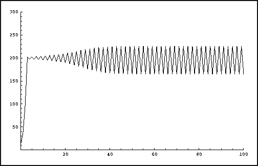
Logistic growth with growth factor
= 3.1.
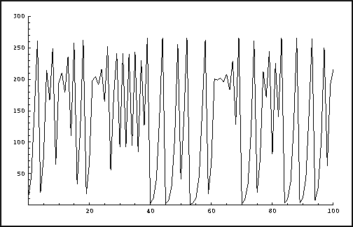
Logistic growth with growth factor
= 4.
Up: Logistic Growth Model
![[HOME]](/pix/home.gif) The Geometry Center Home Page
The Geometry Center Home Page
Written by Hinke Osinga
Comments to:
webmaster@geom.umn.edu
Created: Apr 1 1998 ---
Last modified: Wed Apr 8 18:10:03 1998