
The basic idea is essentially the same as the standard predictor
corrector algorithm:
1) find one point on the curve;
2) compute a tangent vector to the curve at that point;
3) step out a small amount along the tangent vector;
4) relocate the curve at a new point, and store the singular data
for later use;
5) go to step (2).
We want to emphasize that the singular curve (if it exists) is the solution of the over-determined system of the equations:
f=0,Let F be the function F=(fx,fy,fz), then DF=hessian of f. If x0 is a solution of the system above and if DF(x0) has full rank, then x0 is an isolated solution. So if there is a solution curve passing through x0, DF(x0) must have rank less than 3. In the case that rank(DF(x0))=2, the tangent space to the singular curve at x0 coincides with the null space of DF(x0). (We actually use this fact to process step (2).) Currently we assume that rank(DF(x0))=2 except at finitely many points.
fx=0,
fy=0,
fz=0.
In order to accomplish step (1), we first use Newton's method on the system formed by F to find roots of F. Each root is a candidate solution to (f,F)=(0,0). As we attempt to iterate onto the singular curve, Newton's method will eventually complain at some point, say xk, since DF has rank less than or equal 2 along the singular curve. In this case, we restrict our searching for a candidate on the plane passing through the point xk and orthogonal to the null space of DF(xk). After we find a candidate, we then check to see if we really found a point on the singular curve or not. That is, we verify that f=0 and F=0.
For instance, let f=x2 - y2 then F=(2x,-2y,0) and DF is the diagonal matrix with 2, -2, and 0 on the main diagonal. Note that DF has always rank 2. Newton's method can not apply to the system F=0 to find the solutions. However the first two rows of DF are linearly independent and (0,0,1) is a vector in the null space of DF. So with an initial guess (a,b,c) we try to solve the system
2x=0,Therefore we find the candidate (0,0,c). Finally, we verify that f=0 and F=0, which are true. So we found a point on the singular curve.
-2y=0,
(x-a,y-b,z-c).(0,0,1)=0, that is z-c =0.
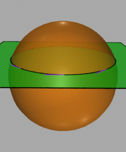
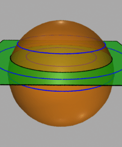
If we encounter a point x0 on the curve with rank(DF) less than or equal to 1, then we will compute the intersection curves of the zero surface f=0 and a sphere of suitable size centered at x0. We will do the same thing for isolated singular points. This will help us to understand the local structure near those singular points.
In step (2), as we mentioned above, we use the null space of DF(x0) to compute the tangent of the singular curve at x0.
For steps (3) and (4), we pick two equations from the system F=0, based on which two row vectors of DF(x0) are linearly independent. Then we add the third equation: (x - w0) . T0 = 0 to make up a non-degenerate system, where w0 = x0 + step_length * T0 and T0 is a unit tangent vector at x0. Now we use Newton's method again to relocate a new point onto the curve using the new system of equations (of course, we need to check to see if we really got a solution for the original system or not).
We remark that we save the singular curve as a list of arcs for later use. Each arc contains a list of points on the singular curve and tangent vectors at each point.

To fill in the local structure, we do the following
1) form a cylinder around the singular curve;
2) trace the boundary curve (the intersection of the level set
and the cylinder), and store the data for the regular two-parameter
continuation to trace the rest of the level surface;
3) triangulate the surface between the boundary curve and the singular
curve.
Assume that s(t) is a parameterization of the singular curve. Then the cylinder of radius r in step (1) may be characterized by
(x-s(t)).(x-s(t))-r2=0;where x is a point on the cylinder. So the boundary curve can be defined by
(x-s(t)).s'(t)=0;
(x-s(t)).(x-s(t))-r2=0;Note that the domain of the system is four dimensional (including t) and the range is three dimensional. Recall also that we already stored the singular data, so we can calculate s(t) and s'(t) by linear or quadratic interpolation for any given t. This is the perfect situation to apply the standard predictor-corrector algorithm.
(x-s(t)).s'(t)=0;
f(x)=0.
We trace the boundary curve "arc by arc" as we traverse the singular curve. For example, let x0 and x1 be two end points of an arc on the singular curve. Let T0 and T1 be unit vectors tangent to the singular curve at x0 and x1 respectively. Finally let S0 and S1 be the circles of radius r, centered at x0 and x1 and perpendicular to T0 and T1 respectively. Then we use the points that are on S0 and S1 and simultaneously are on the zero surface of f as the initial points to trace parts of the boundary curve. The computation of these points reduces to a one dimensional root finding problem. So we can use a "bisection method" to find roots. The rest of step (2) is standard.
The meaning of the five parameters below is pretty much the same as the standard predcorr algorithm. They were documented in detail in the documentation for the Predictor-Corrector Algorithm.
| 1. Step_Length | Default value: 0.02 |
| 2. Max_Steps | Default value: 120 |
| 3. Random_Points | Default value: 0 |
| 4. Selected_Points | Default value: 0 |
| 5. Uniform_Points | Default value: 3 |
The following parameters are specific to Sing3D algorithm.
| 6. Display_IP | Default value: 1 |
| 7. Radius | Default value: 0.3 |
| 8. Zero_Vector_Tol | Default value: 0.001 |
| 9. Boundary_Smoother | Default value: 1.5 |
| 10. Circle_Division | Default value: 100 |
| 11. Trace_Boundary_Curve | Default value: 1 |
![[Pisces]](../../../pix/pi.gif) The Pisces Home Page
The Pisces Home Page