More Complicated Models of Experimental Data
There are obvious problems with the PL and PC models that we have been
using. For example, many processes occur smoothly, so it may be
important to choose a model which has no breaks or kinks. For other
processes, we may want to choose a model which is periodic (that is,
it repeats itself) or which has a certain number of derivatives. In
this section we introduce a few new models that may be used to
approximate functions underlying experimental data. In each case, we
can approximate the integral of the (unknown) function underlying the
data by exactly integrating the (known) model of our choice. It is
often the case that the choice of "the best" model to use is not made
on mathematical grounds, but is made by knowing something about
physics, biology, economics, or some other disciplne.
Modeling Data Sets
Given a data set, each of the functions below is often used to model
the (unknown) function underlying the data. The interactive
document on the next page allows you to select a model for the pollution-rate
data presented in Figure 2.
A little notation will be useful. Suppose that you have n pieces of data.
The data was recorded at times
t0, t1, t2, ..., tn and the corresponding measurements
were P0, P1, P2, ..., Pn.
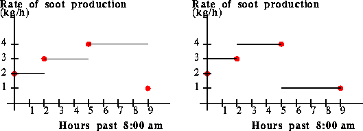
Piecewise Constant: Left Hand Rule
For any instant in time between t0 and t1, the value
of the (left hand) piecewise constant model is P0. For any
instant between t1 and t2, the value of the model is
P1, and so on.
We need to make an assumption about how to define the model for time
less than t0 or time greater than t1. We will make
the simplest assumption: the model is always zero for times prior to
t0 or for times greater than tn.
Piecewise Constant: Right Hand Rule
This model is similar to the previous model, except that for any
instant in time between t0 and t1, the value of the
(right hand) piecewise constant model is P1. For any instant
between t1 and t2, the value of the model is
P2, and so on.
The extension of the model outside of the range of data is the same as
above.

Figure 4: The graph of two piecewise constant models
for the "pollution-rate function" over the interval [0,10.5].
Question 5
Above, you were given the definition of two piecewise constant models.
Now it is your turn to construct a
definition of a piecewise linear model. This model
is linear between two data points.
Construct a formula, valid for any set of data points,
that explicitly gives the value
of the model when the input is between t0 and t1,
between t1 and t2, and so on.
Extend the model outside of the range of data in the same way as for
the previous models.
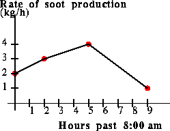
Test your model on the "EPA
data" shown in Figure 2. For this data, the graph of your
piecewise linear model looks like the Figure below.

Figure 4: The graph of a piecewise linear model
for the "pollution-rate function": time versus rate of soot
production.
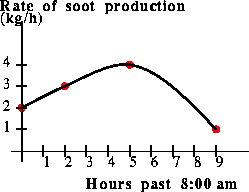
Cubic Spline
This model is used by engineers and architects in order to fit a
smooth curve to a set of data points. The model is a cubic polynomial
on each interval between data points. (The model is not,
however, a cubic polynomial over its entire domain!) The cubic
polynomials are chosen in such a way as to make the derivative of the
model be continuous over the entire domain.
The extension of the model outside of the range of data is the same as
the other models, but the fact that we are fitting a cubic polynomial
to the data set gives us additional freedom. In this lab, we have
chosen the cubic polynomial so that the slope of the model at
t0 is the slope of the line segment from (t0,P0) to
(t1,P1). Similarly, the slope of the model at tn is
set to be the slope of the line segment from
(t_(n-1),P_(n-1)) to (tn,Pn).
We will see examples of these models in later portions of the lab.

The graph of a cubic spline
model.
Trigonometric Polynomial of Best Fit
You may know that it is possible to write down the equation of a line
that best fits a set of data points. Similarly, it is possible to
write down the equation of a quadratic function, a cubic function, or
any other polynomial of a fixed degree that "best fits" the given
data. The exact way to do this is often presented in a course in
statistics or linear algebra; we will not concern ourselves with the
details, but typically "best fit" means looking at the difference
between the model and data points, and then minimizing the sum of the
squares of those differences.
If you suspect that the data you are gathering is periodic over some
interval of time, then it may make sense to choose your model to be
periodic as well. In analogy to the "polynomials of best fit," it is
possible to write down a model that consists of a sum of sine and cosine
functions that best fit the given data. It is necessary, however, to
decide ahead of time how many sines and cosines you want to use in
your approximation, just as it is necessary to decide on the degree of
the polynomial model that you are fitting to the data.
The models that consist of trigonometric functions are called
Fourier polynomials. These models are widely used in
engineering, physics, and other sciences to approximate processes that
are periodic.
As an example, suppose that the EPA worker knows that the factory that
he is testing runs two twelve-hour shifts. The worker suspects that
the rate of soot production may be periodic over a twelve hour period.
The simplest Fourier polynomial of "best fit" is then
2.5 - 0.775 cos(w t) + 1.342 sin(w t)
where w= 2 Pi/12 = Pi/6.
More complicated models (higher "degrees") could include trigonometric
functions like sin(2 w t), cos(2 w t), and, in general,
sin(k w t) and cos(k w t) for any integer value of
k. For example, the best-fit Fourier polynomial of degree-two is
2.5 - 0.732 cos(w t) + 1.268 sin(w t) + 0.232 cos(2 w t) - 0.134 sin(2 w t).
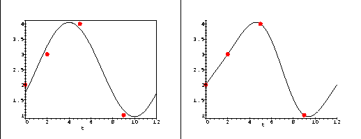
Note that Fourier polynomial we produced is periodic over the
time interval [0,12]. The comparison of this function with the
experimental data is shown below.

Figure 5: The graph of a Fourier polynomial model
for the "pollution-rate function," assuming the data has
a 12 hour period, beginning at t=0.
(A) The Fourier polynomial of
degree one that best fits the experimental data.
(B) The Fourier polynomial
of degree two that best fits the data.
Summary of Models
There are many ways to model the unknown pollution-rate function.
Each model has certain advantages and disadvantages, and in practice scientists
try to choose a model whose characteristics best reflect what is known about the
underlying function. In the remainder of this lab, we apply these models to
two sets of experimental data.
Next:Models of CO2 Concentrations in a River
Previous:Models of Experimental Data
Return to:Introduction
The Geometry Center Calculus Development Team
A portion of this lab is based on a problem appearing in
the Harvard Consortium Calculus book, Hughes-Hallet, et al,
1994, p. 174
Last modified: Wed Feb 21 13:10:29 1996
