Models of Experimental Data
Let's think about the problem of integrating the experimental data
gathered by our hypothetical EPA worker. The first thing is that we
have to accept the fact that we do not know the
underlying function that, for each instant of time, gives the rate at
which soot is being produced at that instant. There is no possible
way to know the underlying "pollution-rate function"; the best we can hope
for is that our data gives us a good idea of this function.
Note that the "pollution-rate function" is a rate; to obtain the amount of
pollution, we need to integrate the pollution function.
Question 1
-
With the current data, determine your best guess for the rate of soot
production at 3:00 pm. What assumptions did you use in order to come
up with that guess?
- Suppose the EPA worker comes back with an electronic device that
measures the factory's rate of soot production at 20 minute intervals,
beginning at 8:00 am.
- Will this additional data make it easier to know the amount of soot
that the factory is producing? Why or why not?
- If you have access to this new data, explain how you could
approximate the rate of soot production at 3:00, at 3:10, and
at 3:15.
Since we don't have a formula for the "pollution-rate function",
let's try to approximate the integral of this function based on our
understanding of the graphical meaning of the integral and what little
information we do have. The EPA worker measured the pollution-rate function at
four instants of time. We will rewrite the data in a sightly
different form and plot the new data:
    Hours        Measured rate of soot
    after 8:00   production (kg/hour)
    ------      -----------------------
      0                2
      2                3
      5                4
      9                1
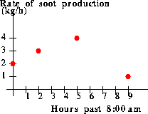
Figure 2: A plot of experimental
data for the "pollution-rate function": time versus rate of soot
production.
There are two especially simple assumptions that we can use to "fill
in" the missing portions of the graph of the pollution-rate function:
the assumption that the pollution-rate function is constant when there
are no data points, or the assumption that the pollution-rate function
is linear between data points.
Question 2
Assume that the pollution-rate function is constant whenever no data is
present. In other words, assume that the rate of soot production is
exactly 2 kg/hour for every instant of time between 8:00 and
10:00, it is exactly 3 kg/hour from 10:00 until 1:00, and so
on. The function that we get by this process is called the
piecewise constant model (or PC model) for the pollution-rate function.
- Plot the piecewise constant model on the domain [0,10]
using the graph provided.
- Graphically represent the area under the graph of the PC model
as a union of rectangles.
- Using geometric techniques, find the exact integral of
the piecewise constant model on this domain.
- According to this model, how many kilograms of soot did the
factory produce during ten hours of operation?
- One advantage to this model is that the integral is relatively
easy to calculate. What disadvantages are there to this model? How
realistic is the assumption that the rate of soot production remains
constant between data points?
Question 3
Assume that the pollution-rate function is linear
whenever no data is
present. In other words, assume that the rate of soot production
increases steadily from between 8:00 and 10:00, increases at a
different steady rate between 10:00 and 1:00, and then decreases
steadily from 1:00 until 5:00. Thus, for example, we will assume that
the rate of soot production at 9:00 was 2.5 kg/h. The function that
we get by this process is called the piecewise linear model
(or PL model) for the pollution-rate function.
- Plot the piecewise linear model on the domain [0,10]
using the graph provided.
You will need to make an additional assumption in order to
graph the PL model on the interval [9,10]. Explicitly state
what assumption you used.
- Graphically represent the area under the graph of the PC model
as a union of trapezoids.
- Using geometric techniques, find the exact integral of
the piecewise linear model on this domain. (Hint: recall the
area of a trapezoid.)
- According to this model, how many kilograms of soot did the
factory produce during ten hours of operation?
- What advantages and disadvantages are there to this model?
Do you think that amount of soot predicted by this model
is more or less valid than the amount predicted by the PC model?
Why?
Question 4
Once again, suppose the EPA worker installs an electronic device that
measures the factory's rate of soot production at 20 minute intervals,
beginning at 8:00 am.
- For the new data, you can still model the pollution-rate function as
piecewise constant or piecewise linear. Do you expect the
differences between the PC and PL models based on this new data
set (with more data points) to be more or less pronounced than for the
original data (the data set with four data points)?
- Suppose now the EPA worker gains access to a device that measures
the factory's rate of soot production at 1 minute intervals.
Show that the integral of the PL and PC models will be nearly identical.
Construct an argument and sketch a diagram
to indicate why the claim is true. (Hint: Look at the area under the
PL model that is not under the PC model.)
Next:More Complicated Models
Previous:A Thought Experiment
Return to:Introduction
The Geometry Center Calculus Development Team
A portion of this lab is based on a problem appearing in
the Harvard Consortium Calculus book, Hughes-Hallet, et al,
1994, p. 174
Last modified: Fri Jan 5 09:51:05 1996