Models of Experimental Data

On occasion, scientists gather experimental data that represents the rate at which some quantity changes. To obtain the net change in the quantity, it is necessary to integrate the underlying data. There is a major difficulty, however. Namely, we do not know the underlying function that, for each instant of time, gives the rate at which the quantity is changing at that instant. There is no possible way to know the underlying "rate function"; the best we can hope for is that our data gives us a good idea of this function. In this section we introduce a few models that may be used to approximate functions that produce experimental data. In each case, we can approximate the integral of the (unknown) function underlying the data by exactly integrating the (known) model of our choice. It is often the case that the choice of "the best" model to use is not made on mathematical grounds, but is made by knowing something about physics, biology, economics, or some other disciplne.

Modeling Data Sets

Given a data set, each of the functions below is often used to model the (unknown) function underlying the data. The interactive document that accompanies this text allows you to select a model for any data set of your choosing.

A little notation will be useful. Suppose that you have n pieces of data. The data was recorded at times t0, t1, t2, ..., tn and the corresponding measurements were P0, P1, P2, ..., Pn.

We have included the following models of experimental data:

The Numerical Integration Lab discusses these models and also a model that uses Fourier polynomials (trigonometric functions). The lab also addresses the issue of error and accuracy: how can we be confident that our numerical integration is a good approximation to the integral of the underlying (unknown) function that gave rise to the experimental data?

The Models

Piecewise Constant: Left Hand Rule

For any instant in time between t0 and t1, the value of the (left hand) piecewise constant model is P0. For any instant between t1 and t2, the value of the model is P1, and so on.

We need to make an assumption about how to define the model for time less than t0 or time greater than t1. We will make the simplest assumption: the model is always zero for times prior to t0 or for times greater than tn.

Piecewise Constant: Right Hand Rule

This model is similar to the previous model, except that for any instant in time between t0 and t1, the value of the (right hand) piecewise constant model is P1. For any instant between t1 and t2, the value of the model is P2, and so on.

The extension of the model outside of the range of data is the same as above.
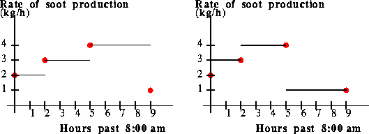

The graph of two piecewise constant models for a "rate function."


Piecewise Linear Models

This model is linear between two data points. In particular, if t is between t0 and t1, then we may write t = t0 + a dt where dt= t1-t0. Then the value of the model at t is defined to be P0 + a dP where dP = P1-P0.

The model is defined similarly for other values of t in the interval for which we have data. As above, the model is assumed to be zero outside of the range of data.
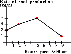

The graph of a piecewise linear model for a "rate function".


Simpson's Rule (Piecewise Quadratic)

Suppose we only have three data points. We can find a quadratic polynomial (a parabola) that passes through each of those data points, and we might choose to say represent the area of the experimental data by the integral of the quadratic function.

If we have an odd number of data points, then we may split up the data points into groups of three: we group together data points 1-3, 3-5, 5-7, and so on. For each triple, we may fit a quadratic polynomial through the data points, and then sum up the areas under each parabola in order to estimate the integral of the experimental data. In the case that the independent variables of the experimental data are distributed uniformly, this method reduces to the well-known Simpson's Rule for numerical quadrature.

If the number of data points is even, then Simpson's rule cannot be directly applied. What we have implemented here is the following scheme: we fit a parabola to the first three data points, and use this to interpolate a new data point whose abscissa lies between t0 and t1. We then add this point to the data set, creating an odd number of data points, and then we proceed as above.

The extension of the model outside of the range of data is the same as the other models.
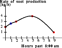

The graph of a piecewise quadratic model. There were originally an even number of data points, so the first three points were used to interpolate a new data point (shown in blue), which was then added to the data set.


Cubic Spline

This model is used by engineers and architects in order to fit a smooth curve to a set of data points. The model is a cubic polynomial on each interval between data points. (The model is not, however, a cubic polynomial over its entire domain!) The cubic polynomials are chosen in such a way as to ensure continuity of the model function's derivative over the entire domain.

The extension of the model outside of the range of data is the same as the other models, but the fact that we are fitting a cubic polynomial to the data set gives us additional freedom. In this lab, we have chosen the cubic polynomial so that the slope of the model at t0 is the slope of the line segment from (t0,P0) to (t1,P1). Similarly, the slope of the model at tn is set to be the slope of the line segment from (t_(n-1),P_(n-1)) to (tn,Pn).
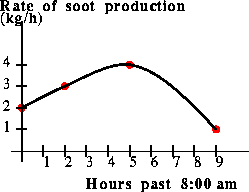

The graph of a cubic spline model.


Summary of Models

There are many ways to model an unknown rate function, based upon knowledge of its value at a few points. Each model has certain advantages and disadvantages, and in practice scientists try to choose a model whose characteristics best reflect what is known about the underlying function.
Previous: Integrating Experimental Data

The Geometry Center Calculus Development Team

Last modified: Fri Jan 31 14:25:46 1997