Overview

How Predictor-Corrector works

1. find one point on the curve;
2. compute a tangent vector to the curve at that point;
3. step out a small amount along the tangent vector;
4. relocate the curve at a new point
5. go to step 2

This particular implementation attempts to intelligently implement this basic strategy by

1. Finding special points on the curve to use as initial starting points for the tracing. These "special points" include
   • turning points (where one of the derivatives to the curve vanishes)
   • boundary points (where f=0 intersects a bounding box)
   • singular points (for planar curves, where f=0 and grad(f)=(0,0))
   We allow the user to select which types of initial points to search for and use. Choices include the special points described above as well as points obtained by iterating onto the curve seeds corresponding to points on a uniform grid, to random points, or to points selected by the user.

2. Detecting and locally resolving planar singularities. By this I mean that we excise a neighborhood of the singularity and replace that region by a local representation of f=0 near the singularity. This uses ideas from singularity theory, differential geometry, and algebraic geometry. For more information on the desingularization algorithm, see that portion of the documentation.

3. As we trace the curve, we keep track of where we are relative to any "special points" we may have computed. If we enter a neighborhood of a special point, then we intelligently connect f=0 to the point.

Controlling the Algorithm from Pisces

Replace this image file

Replace this image file

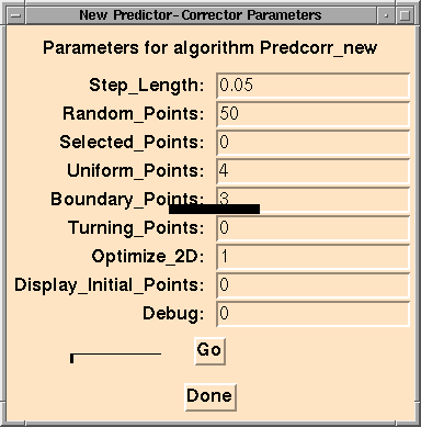
The Pisces panel to the predictor corrector algorithm currently has 9 parameters which may be set from the algorithm window:

1. Step_Length
   This field should contain a positive numerical value. It indicates the step length for the predictor part of the algorithm. That is, we take a step of length Step_Length in the direction tangent to the curve, before using Newton's method to correct back onto the curve. Due to this correction, the actual length of the line segments outputted by the algorithm will vary somewhat at different points along the curve. If Optimize_2D is off or if the model domain is of dimension greater than 2, each segment will have length AT LEAST Step_Length.
   Default value: 0.05

   The following six parameters allow the user to choose among various methods of selecting initial points. At least one of these fields must be nonzero in order to obtain output. Several or all of them may be selected at once.

2. Random_Points
   This field should contain a nonnegative integer value. This value specifies the number of random points (all within the domain boundaries of the model) that the algorithm will generate. Each of these points is then used as a seed for Newton's method, which attempts to iterate these seeds onto the curve. In a model with domain dimension n, these iterations are confined to an n-1 dimensional subspace of the domain in order to obtain a fully determined system. If the random point is p, this hyperplane is chosen as the n-1 dimensional subspace orthogonal to the tangent vector at p to the level curve f(x) = f(p). Newton's method works somewhat differently if n = 2 and Optimize_2D is set to 1. See documentation for Optimize_2D below. Default value: 50

3. Selected_Points
   This field takes a boolean value 0 (false) or 1 (true). If the value is nonzero, the user will be prompted to enter points, coordinate by coordinate, at the Pisces command line. The user is allowed to enter as many points as desired. The algorithm attempts to iterate the points onto the curve using Newton's method.
   Default value: 0

4. Uniform_Points
   This field should contain a nonnegative integer value. A value of 0 indicates that uniform grid points should not be used as seeds. Given a positive value m for Uniform_Points in an n-dimensional model, the algorithm constructs a uniform grid with m^n points, and attempts to iterate each point onto the curve using Newton's method. Specifically, the algorithm divides the domain space into m^n uniform n-cubes, and places a grid point at the center of each cube.
   Default value: 4

5. Boundary_Points
   This field should contain a nonnegative integer value. If the value is positive, the algorithm sets up a grid along each boundary face of the domain space, and attempts to iterate each point onto the curve under the constraint that all points must remain along that boundary. Given a value m for Boundary_Points, the grid used is uniform as described above, with m^(n-1) points per boundary. All initial points found by this method will be along the boundaries.
   Default value: 3

6. Turning_Points
   This field should contain a nonnegative integer value. If the value is positive, the algorithm sets up a uniform grid (where the Turning_Points parameter specifies the fineness of the grid, as described in #4 above), and attempts to iterate each point onto a turning point of the curve with respect to each axis. A turning point is defined as a point where the tangent to the curve either is not uniquely defined (a singularity) or is perpendicular to one of the axes. For each grid point, a separate series of iterations is required for each axis to which a turning point might correspond.
   Default value: 0

7. Singular_Points Not Yet Implemented
   The version of Predcorr_new incorporated in the master copy of Pisces does not yet contain this parameter.

   WARNING: When using models with a large number (n) of dimensions, be careful not to use large values (m) for Uniform_Points, Boundary_Points, and Turning_Points. The values in these fields do not indicate the total number of seeds to use; they represent the fineness of the grid. The functions which find uniform and turning points use m^n seed points, while the one which calculates boundary points uses m^(n-1) seed points per boundary. Large values of Turning_Points (say, above 10 for three or more dimensions) may cause the algorithm to be especially slow, since turning point iterations are relatively complex and since a separate set of these iterations must be executed for each coordinate axis for each point.

8. Optimize_2D
   This field takes a boolean value 0 (false) or 1 (true). The value of this field has no effect unless the model is planar. If this option is turned on and the model is planar, the predictor-corrector algorithm uses a specialized routine for implementing Newton's method, both for determining initial points from random, uniform, or user-selected seeds, and for correcting back onto the curve after taking a predictor step (the specialized functions are not used while searching for boundary points, turning points, or singularities). These functions are referred to as optimized because all formulas are hard-coded for the special case of two dimensions (in which many of the formulas become degenerate). LU decomposition and backsolve routines are not used.

   The 2D "optimized" functions also differ from the general ones (when used for a planar model) in that they use a different variant of Newton's method. These functions are called in cases when Newton's method is in fact being used to solve a system which is underdetermined by one equation. Classically, Newton's method requires a fully determined system (i.e., it involves the inversion of a square matrix). The general procedure solves this problem by introducing the additional condition that the iterations occur within a hyperplane perpendicular to a previously determined vector (the vector used is typically a tangent vector; when stepping along the curve, it is the vector indicating the direction in which the step was taken). The "optimized" functions do not add this extra condition; they implement Newton's method on an underdetermined system, using the method of the Moore-Penrose inverse described in Allgower and Georg. For the planar case, this simply involves recomputing the gradient at each iteration, and taking a Newton's step in that direction. Our experimentation shows that (after we fixed a seemingly endless string of bugs in these optimized functions) the optimized functions tend to give better results than their general counterparts, and to execute slightly faster. However, the behavior of the optimized functions is sometimes less predictable, and we have found a few cases where the general functions gave better results.
   Default value: 1

9. Display_Initial_Points
   This field should contain either 0 (false) or 1 (true). If it is 0, only the actual curve computed by the algorithm will be displayed. When this field is set to 1, the initial points that were used to trace the curve will also be displayed as red dots. In addition, the algorithm will output its bounding box (separate from Geomview's bounding box) in black when this option is set.
   Default Value: 0

10. Debug
    This field should contain either 0 (false) or 1 (true). When Debug is 1, a very large quantity of unimportant information will be displayed on the standard output. This output describes whether or not Newton's method successfully converged to each initial point, and how the line segments were traced between the initial points. This option is not intended for general use, although some people find the debugging output strangely interesting.

    There are also some graphical effects when Debug is set to 1. After the algorithm computes all of its initial points, it selects an appropriate subset of those initial points to be used in the tracing of the curve. When both Display_Initial_Points and Debug are set to 1, the initial points that were NOT selected to be used to trace the curve will also be displayed. Points that were too close to another point will be displayed as blue dots, and points that were outside of the bounding box will be displayed in green.

    If you want your X server to spend minutes on end outputting text debugging information, then try setting Debug to 2 (which will output everything you get with Debug set to 1, and more).
    Default Value: 0

Known Bugs

1. Unimplemented features
2. Output bugs

In the future, we plan to add singularity handling, desingularization for planar singularities, and an adaptive step length to the new Predictor-Corrector algorithm. Currently, your results will vary considerably when you try to plot singular curves.

More likely than not, you will also have the wonderful privilege of encountering one of the known output bugs. None of these bugs are intrinsic to the new Predictor-Corrector algorithm; they are all caused by other portions of the Pisces code or by Geomview. If you use Geomview as your output device, you will occasionally be informed that Geomview can't seek back far enough on its input pipe. This bug will probably not be fixed any time soon. There is also a bug relating to the handling of polyline objects in the geomview interface code; this bug occurs much more frequently, but it will hopefully have been fixed by the time you read this.

Bug Reports

Algorithm Implemented By

The great and almightly summer students are

• Erik Streed streed@geom.umn.edu
• Ron Dror dror@geom.umn.edu
• John Golden jgolden@geom.umn.edu
• Brian Johnson bwj@geom.umn.edu

Acknowledgements

The Geometry Center Home Page

Comments to: pisces@geom.umn.edu
Created on Thu Jun 8 09:02:40 CDT 1995 by Fredrick J Wicklin
Converted to html on July 28, 1995 by Erik Streed
Last Modified: July 28, 1995
Copyright © 1995 by The Geometry Center, all rights reserved.