Up to Pisces Online Documentation

Adaptive Grid 2D Algorithm

( AGrid )

Overview

This algorithm locates a level set of an arbitrary 2D function. It should locate all components of the level set, even fairly small ones, and treats singularities well (though not perfectly).

How Adaptive Grid Works

A traditional method of locating the zero set of a function is to break the domain into a grid (like graph paper), and then for each square in the grid, look along the edges of the square for zeros of the function. This is usually done by evaluating the function at the corners of the square and looking for edges that have a sign change; provided the function is continuous, there will be a zero somewhere along such an edge. The position of the zero is approximated using the values of the function at the corners, usually via linear interpolation. Once the positions of the zeros along the edges of the squares are located, these zeros are joined by line segments through the interior of the square. Taken over all the squares in the grid, these line segments represent an approximation to the actual zero set of the function. To get a better approximation, one uses a finer grid.

The main drawback of this approach is that in order to obtain improved resolution, the grid must be made finer over the entire domain, including part of the domain that are far from the zero set, so a lot of work will be done even where it is unnecessary. The main idea of AGrid is to begin with a fairly course initial grid, and then refine it only where it is necessary. This allows for higher resolution in the neighborhood of singularities, for example, while still allowing for lower resolution in places where the level curve can be represented adequately by longer linear segments.

An algorithm of this sort requires a subdivision criterion that determines when a portion of the grid should be divided, and when subdivision is no longer necessary. AGrid employs several different tests in order to decide if a subdivision is needed, and these are divided into three groups: tests based on the behavior of the function along the edges of the grid; tests based on the line segments used to approximate the zero set within a region of the grid; and tests based on the subdivisions occurring within neighboring regions of the grid. If any of the tests along any edge of the region requires subdivision, the region is subdivided. Likewise, if the approximation to the zero set requires more subdivision, or if the neighboring regions suggest that subdivision is needed, then the region will be subdivided, otherwise it is no longer divided and the approximations to the zero set that it contains are added into the final representation of the zero set. The tests themselves are controlled by the parameters described below.

Controlling the algorithm from Pisces

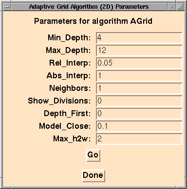
The AGrid algorithm uses a triangular mesh which is obtained by taking a rectangular domain and dividing it into two triangles. Each of these triangles is then subdivided, and the resulting triangles subdivided again, and so on for a total of MIN_DEPTH times (giving 2*2^MIN_DEPTH initial triangles). A setting of 4 gives a good starting configuration.

MAX_DEPTH gives the maximum number of times that a triangle will be divided. That is, if a triangle is the result of subdividing one of the initial triangles MAX_DEPTH times, then it will not be subdivided further even if the other tests say it should. Setting MAX_DEPTH equal to MIN_DEPTH makes AGrid work essentially like the traditional (non-adaptive) algorithm. A value of around 12 to 15 is usually sufficient.
SHOW_DIVISIONS takes a value of 0 or 1, with 1 meaning that AGrid will output the boundaries of the triangles that it has used in the grid, and 0 meaning that the triangles are not shown. This is sometimes useful as a means of seeing where AGrid is spending most of its energy, particularly as you try to adjust the other parameters.
DEPTH_FIRST takes a value of 0 or 1, with 1 meaning that each triangle is divided to as small as it needs to be before the next triangle is processed, while 0 means that all the triangles of a given size are handled before smaller triangles are processed. Ideally, the results should be the same, but if NEIGHBORS is set to 1, the amount of processing time may be affected.
NEIGHBORS takes a value of 0 or 1, with 1 meaning that subdivisions in one triangle may cause subdivision in neighboring triangles, while 0 means that subdivisions do not propagate to neighboring regions. The idea is that if great detail is needed in one area, then we need to treat the nearby area with more care. Setting NEIGHBORS to 1 can cause the results to be more accurate, and allows the other parameters to be less strict, but at the cost of causing more work to be done when it might not really be necessary. The actual test performed is: if a region is being subdivided and its neighbor is more than twice the size of the resulting triangles, then the neighbor will be subdivided as well. Such subdivisions may propagate outward to neighbors that are farther away, as well.
The ABS_INTERP and REL_INTERP parameters control how accurate an interpolated zero must be in order to be considered good enough to use. When the endpoints of an edge have different signs, the location of the zero between them is approximated by linear interpolation between the values of the function at the endpoints of the edge. The value of the function at this point is computed and checked to see how close it is to zero; if it is greater than ABS_INTERP in absolute value, then it is not considered to be good enough, and the triangle will be subdivided. Otherwise, the value is compared to the average of the absolute values of the values of the function at the endpoints; if the proposed zero is less (in absolute value) than REL_INTERP times the average of the endpoints, then the zero is accepted, otherwise the triangle will be subdivided. A zero must pass both tests in order to be considered accurate. The reason for REL_INTERP is that on an edge where the value of the function is uniformly small, more accuracy is needed when determining the zero, so we test for zero relative to the values of the function nearby, and we always require the zero to be within ABS_INTERP, regardless.

If the zeros along the edges of a triangle all pass these tests, then an approximation to the zero set within the triangle is given by the line segment joining the zeros on the boundary edges. Before this approximation is accepted, it is also tested for accuracy; its midpoint is determined, and the function value at this point is calculated, and it is tested against ABS_INTERP, and REL_INTERP (here the average of the absolute values of the function at each of the corners of the triangles is used for comparison). If the value passes both tests, then the approximated zero set is accepted, otherwise the triangle is subdivided.

Reasonable values for ABS_INTERP and REL_INTERP depend on the function you are actually using, but 0.01 for ABS_INTERP and 0.05 for REL_INTERP make good starting places. Set SHOW_DIVISIONS to 1 and increase the values if subdivisions are occurring where they are not needed, or decrease them if not enough division occurs near the zero set.

For an edge where the sign of the function differs on the endpoints, we know there is a zero somewhere on the edge; but if the signs are the same, there still might be a zero on the edge, so we need a criterion for when to subdivide such edges. First, we compute a point on the edge that is likely to be where the function is closed to zero along the edge (this calculation is based on the values of the function at the endpoints). The function is evaluated at this point; if its sign is different from that at the endpoints, then the triangle will be subdivided. Otherwise, the value is divided by the length of the edge; if the result is greater than MAX_H2W, then the function is considered to be too far from zero over that edge, and we assume there is no zero along that edge, so no subdivision is required. Otherwise, we compare the value of the function at that point to the value of the linear function connecting the values at the endpoints of the edge; if these differ by more than MODEL_CLOSE times the width of the edge, then the triangle will be subdivided. The idea here is that we are using a linear approximation to model the actual function, and if it is close enough to the value of the function, then the fact that the linear model doesn't have a zero indicates that the actual function doesn't have a zero on the edge. (The actual formula used is a bit more complicated than the one given above, and is explained in detail in the complete documentation for the algorithm.)

Reasonable values for MAX_H2W and MODEL_CLOSE depend on the actual function you are using, but values of 2 for MAX_H2W and 0.1 for MODEL_CLOSE are good starting points. Decreasing either of these parameters will cause more subdivisions to occur. Note that ABS_INTERP and REL_INTERP only come into play on edges where the function values at the endpoints have opposite signs, and MODEL_CLOSE and MAX_W2H only come into play when they have the same sign.

Known Bugs

None?

Bug Reports

software@geom.umn.edu

Algorithm Implemented by

Daniel B. Krech

Acknowledgements

Dan Krech not only implemented the algorithm, but also developed the portion of the algorithm that subdivides a triangle based on the size of its neighbors.

This code is based on an algorithm developed by Davide Cervone at the Geometry Center, though this implementation does not include all the features of the complete algorithm. The full algorithm uses tangent information to improve the results, and to locate and identify singularities and non-transverse zeros.

The Pisces Home Page

The Geometry Center Home Page

Comments to: pisces@geom.umn.edu
Created: Tue Jun 6 16:27:25 CDT 1995 by Davide Cervone
Converted to html on July 25, 1995 by Erik Streed
Last Modified: July 25, 1995
Copyright © 1995 by The Geometry Center, all rights reserved.