This worksheet does not need to be handed in, but you are responsible
for the material. The ideas laid out here will be used in next week's
lab (which will be graded). Some of the instructions for this lab are
taken from J. C. Polking, MATLAB Manual: Ordinary Differential
Equations, Prentice-Hall, 1994.
Gradients appear everywhere in nature. Newton's law of graviation
involve the gradient of a ``gravitational potential function.'' The
equations of electromagnetism (Maxwell's equations) and fluid dynamics
(Navier-Stokes equations) also involve gradient terms. Furthermore,
gradient differential equations are used in science and engineering to
optimize functions of several variables. Understanding the geometry of
gradients is one of the most important goals of this course.
The purpose of the lab is
- to learn how to numerically produce solutions to a planar
differential equation using Matlab and PPLANE.
- to explore the geometry of gradient differential equations.
- to better understand the distinction between graphs and images
of functions.
In this lab we will study gradient flows while simultaneously
learning to use PPLANE.
To get started, invoke matlab by typing
matlab in a Unix shell window.
When the matlab prompt appears, type pplane
to launch the ``phase plane'' module.
The PPLANE Setup window will appear.
In this lab we will examine the gradient flow for the following
function:

This function contains several critical points of varying types.
The gradient flow of a function f is the differential equation defined
by 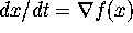 ,
,  . For functions of two
variables, this can be rewritten as
. For functions of two
variables, this can be rewritten as

Since the gradient vector always points in the direction in which f
increases the fastest (or, more correctly, the direction in which the
linear approximation to f increases the fastest), trajectories in a
gradient differential equation ``flow uphill.'' You can think of the
trajectories as the paths in (x,y)-space traced out by a robot that
is programmed to always walk in the steepest direction.
For our example function, 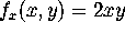 and
and
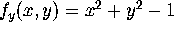 . Therefore the gradient differential equation
determined by the function f is
. Therefore the gradient differential equation
determined by the function f is

Note that for each point (x,y), the right-hand side of the
differential equation, 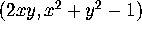 , defines a vector. We therefore
say that the right-hand side of the differential equation defines a
vector field.
, defines a vector. We therefore
say that the right-hand side of the differential equation defines a
vector field.
Activity: Sketch the graph of the current function over the
domain  and
and  (you may use Maple if
you wish). If possible, locate
critical points of the function. Identify where the function is
high and where it is low.
(you may use Maple if
you wish). If possible, locate
critical points of the function. Identify where the function is
high and where it is low.
PPLANE has a default differential equation. Delete it, and type the
right-hand side of the differential equation above into the first two fields of the
PPLANE Setup window. In the lower-left corner of the setup window,
change the minimum and maximum values of the display window to
and . Now hit the Proceed
button and the PPLANE Display window will appear.
Inside this window is a representation of the vector field for this
differential equation. The vector field at (x,y) must be tangent to
the solution curve passing through (x,y). To compute and plot a
solution curve from an initial point, move the mouse to that point,
and click the left mouse button. The solution will be computed and
plotted: first in the direction of increasing time, then in the
direction of decreasing time.
Activity: Compute eight or ten trajectories starting at
different initial conditions (This is called a ``phase portrait.'')
Do the trajectories flow uphill?
Can you use the trajectories to help you locate minima and maxima of
the surface? Are there any critical points not ``located'' by the
trajectories? If so, what do these critical points look like (max/min/saddle)?
Activity: Evaluate the gradient at each critical point that you
find analytically. What is the magnitude of the gradient at a
critical point?
Activity: Suppose you start a trajectory exactly at a critical
point; what does the trajectory look like? Does the shape of the
trajectory depend on the type of critical point? Let's test your guess.
Erase all solutions by choosing the appropriate entry under the
PPLANE Options menu of the PPLANE Display window. Under the
same options menu, start a trajectory at the exact location of a
critical point by choosing the ``Keyboard Input'' menu entry. A small
window will appear; type in the location of a critical point and then
press the Compute button to generate a trajectory starting from
that point. (If ever a trajectory looks different than you expect, ask
yourself ``who is correct'', you or the computer? When doing
numerical experiments, DO NOT assume that the computer is always
correct!)
Activity: For a vector field, places where the vector field is
equal to the zero vector are called equilibria. Use PPLANE to help you
numerically find an equilibrium point (look under the Options menu). When the
vector field is the gradient field for some function, what
is the relationship between ``zeros'' of the vector field and critical
points of the function?
Activity: Use the ``zoom in'' feature of PPLANE to zoom in on
(1) places where the vector field is not zero and (2) places where the
vector field is zero. Based on your experiment, schematically
represent what a gradient vector field looks like
- away from a critical point
- near a maxima
- near a minima
- near a saddle point
(To ``un-zoom,'' retype
and into the lower-left corner of
the setup window and hit Proceed.)
A trajectory is a parametrized curve,  , such that the
tangent vector to the curve at
, such that the
tangent vector to the curve at  is exactly equal to the
vector field evaluated at . Thus differential equations
give us another opportunity to study parametrized curves.
is exactly equal to the
vector field evaluated at . Thus differential equations
give us another opportunity to study parametrized curves.
Note that once a trajectory is numerically
determined, we can view the trajectory in several ways:
- as a parametrized curve in the (x,y)-plane. (This is what we
have been doing so far today).
- as the graph t versus x(t) and the graph t versus y(t).
- as the graph of the function
 in three-dimensional space
The first point of view is the view adopted in dynamical systems,
and leads to a rich geometric understanding of differential
equations. This is the point of view we will typically use in this class. The
second point of view is used when it is possible to explicitly solve
a differential equation for the functions x(t) and y(t). We will
see some of this in the next quarter of this course. The third point of view unites
the previous two views, and leads to a better understanding of the
difference between ``graph'' and ``image.''
Activity: Locate a trajectory that approaches a maximum.
Under the Graph menu of the PPLANE Display window, select
``Both.'' PPLANE will ask you to select a trajectory; do so by
clicking on the trajectory with the left mouse button.
The program will display t versus x(t) and t versus y(t) on
the same graph.
- as t increases, what value does x(t) approach?
- as t increases, what value does y(t) approach?
- What do these two values mean geometrically?
Activity: Now change the graph to ``Composite.''
Look carefully at the axes. What is being displayed?
How does this graph show the relationship between
the graphs of x(t), y(t) and the image of the function that maps
t to (x(t),y(t))?
About this document ...
Return to Labs Homepage
Return to Calculus 3353/3354 Homepage
URL: http://www.geom.umn.edu/~math335x/Labs/Lab04/Lab04.html
Copyright: 1996 by the Regents of the University of Minnesota.
Department of Mathematics. All rights reserved.
Comments to:
hesse@math.umn.edu
Last modified: Oct 23 1996
The University of Minnesota is an equal opportunity educator and employer.